Metropolis-Hastings MCMC from Scratch ✨

Generated with DALL-E

But first, What is Bayesian Statistics? §

If not already clear, Markov Chain Monte Carlo (MCMC) is a tool for implementing Bayesian analyses. Pardon me? If that doesn’t make sense, please stay with me; otherwise, please skip ahead.

Bayesian statistics is just an alternative paradigm to how students are usually first taught statistics, called Frequentist Statistics.

While some might debate you on this, a common perspective is that neither Bayesian nor Frequentist statistics is necessarily better; what’s most important is one recognizes that they are different in implementation but, more importantly, different in their philosophy, the nuances of which will not be covered here. While Frequentist vs Bayesian Statistics is an important discussion, it is also not something you can knock out in 5 minutes. For an extremely brief comparison, see the table below on the difference in Frequentist vs. Bayesian statistics.

 

Bayesian vs. Frequentist Statistics

	Frequentist	Bayesian
Answer given	Probability of the observed data given an underlying truth	Probability of the truth given the observed data
Population parameter	Fixed, but unknown	Prob. distribution of values
Outcome measure	Probability of extreme results, assuming null hypothesis (P value)	Posterior probability of the hypothesis
Weaknesses	Logical inconsistency with clinical decision-making	Subjectivity in priors' choice; complexity in PKPD modeling
Strengths	No need for priors; well-known methods	Consistency with clinical decision-making
PKPD application	Good estimates with large data	Adaptation of data to individuals

(Introna, Michele, et al, 2022)¹

 

What is MCMC? §

MCMC - for the sake of keeping things simple - is a means of sampling a target distribution to arrive at empirical posterior marginal distributions for our parameters of interest, where the target distribution is the distribution that we assume the population response to be following. What’s Notable about MCMC is that it does not require an envelope to sample the target distribution due to the Markov property. In addition, with MCMC, we can arrive at empirical posterior marginal distributions for the parameters of interest without needing conjugate priors.

Practically, this means there is ample software people can use to do Bayesian analysis using MCMC without needing to know the statistical theory that allows for it to work in the first place. With regard to reducing barriers to entry, this is a big deal! However, understanding how algorithms work is crucial! It helps data scientists make informed decisions about the choice of models and algorithms, ensuring the robustness and accuracy of their analyses. Moreover, Understanding the underlying mechanics of MCMC also aids in diagnosing convergence issues and interpreting the results correctly.

Now, on with the post!

 

Agenda

The purpose of this post is to demonstrate how to implement the Metropolis-Hastings MCMC algorithm from scratch for a multiple linear regression.

The First implementation will be designated implementation (a); after that, I will add more complexity but also realism in implementations (b) through to (c), mirroring something closer to canned software such as Jags and BUGS. Let’s break down some of the first steps.

 

MCMC Outline §

1. Sample a candidate value ${\mathbf{X}}^{\ast }$ from a proposal distribution $g\left(\cdot \mid {\mathbf{x}}^{(t)}\right)$.
2. Compute the Metropolis-Hastings ratio $R\left({\mathrm{x}}^{(t)},{\mathbf{X}}^{\ast }\right)$, where

$$R(\mathbf{u},\mathbf{v})=\frac{f(\mathbf{v})g(\mathbf{u}\mid \mathbf{v})}{f(\mathbf{u})g(\mathbf{v}\mid \mathbf{u})}.$$

Note that $R\left({\mathrm{x}}^{(t)},{\mathbf{X}}^{\ast }\right)$ is always defined, because the proposal ${\mathbf{X}}^{\ast }={\mathrm{x}}^{\ast }$ can only occur if $f\left({\mathrm{x}}^{(t)}\right)>0$ and $g\left({\mathrm{x}}^{\ast }\mid {\mathrm{x}}^{(t)}\right)>0$. 3. Sample a value for ${\mathbf{X}}^{(t+1)}$ according to the following:

$${\mathbf{X}}^{(t+1)}=\{\begin{array}{ll}{\mathbf{X}}^{\ast }& \text{ with probability }\min \left\{R\left({\mathbf{x}}^{(t)},{\mathbf{X}}^{\ast }\right),1\right\},\\ {\mathbf{x}}^{(t)}& \text{ otherwise. }\end{array}$$

4. Increment $t$ and return to step 1.

(Givens and Hoeting, 2006)²

 

Writing our first MCM for implementation (a) §

1. Read in Data
2. Write our own Sample Function
3. Specify Likelihood Function
4. Use Optimisation to Get Starting Values
5. Specify Prior Function
6. Specify Posterior Function

Once these five steps are completed, we can begin to write the MCMC algorithm.

1. Reading in the Data §

library(here)
dat = read.csv(here("data","bodyfat.csv"));n = nrow(dat)
y = dat[,1]; X = as.matrix(cbind(Int = rep(1,n),dat[,-1]))
p = ncol(X); n.s = 100000; k = p - 1; ee = 1e-16
par_names <- c(paste0("beta_", 0:13),"sigma_sq")

 

The data is on the percent body fat for 252 adult males, where the objective is to describe 13 simple body measurements in a multiple regression model; the data was collected from Lohman, T, 1992³ .

Potential Predictors of Body Fat - Data from Lohman, T, 1992

1. Age (years)	8. Thigh (cm)
2. Weight (pounds)	9. Knee (cm)
3. Height (inches)	10. Ankle (cm)
4. Neck (cm)	11. Extended biceps (cm)
5. Chest (cm)	12. Forearm (cm)
6. Abdomen (cm)	13. Wrist (cm)
7. Hip (cm)

2. Write our own Sample Function §

Later, we will need a function to summarise the results from the posterior distributions, see samp.o.

samp.o <- function(t.s) {
  round(
    c(mean = mean(t.s),
      sd = sd(t.s),
      lower = quantile(t.s, 0.025, names = F),
      upper = quantile(t.s, 0.975, names = F)), digits = 6)
}

Now we have our data, we need to specify a Likelihood Function.

 

3. Specify Log-Likelihood Function §

Because we have a numerical response, it is reasonable to assume that our population resposne is normally distributed:

$$Y\sim \text{N}(\mu ,{\sigma }^2)$$

Note, that we are using Log Likelihood for numerical precision.

llike <- function(pars) {
  beta <- pars[1:(length(pars)-1)]
  sigma_sq <- max(pars[(length(pars))],ee)
  sum(log(dnorm(y, mean = X %*% beta, sd = sqrt(sigma_sq))))}

Next, we need to get estimates to use as our starting values as MCMC is sent to where they start chains for each parameter.

 

4. Use Optimisation to Get Starting Values §

par0 = c(mean(y),rep(0,p-1),3)
opt <- optim(par = par0,fn = llike,method = "BFGS",
             hessian = TRUE,control = list(fnscale=-1))
np <- length(opt$par)
opt$par

beta_0	beta_1	beta_2	beta_3	beta_4	beta_5	beta_6	beta_7	beta_8	beta_9	beta_10	beta_11	beta_12	beta_13	sigma_sq
-17.8	0.057	-0.086	-0.037	-0.43	-0.018	0.89	-0.196	0.236	-0.021	0.167	0.157	0.429	-1.47	15.1

Note

These estimates are very similar to what you get with coef(lm(y ~ ., data = dat))

 

5. Specify Prior Function §

Using the Jeffreys prior (an improper prior), we can implement a Random Walk Chain with Metropolis-Hastings Markov Chain Monte Carlo to sample the Normal target distribution where Jeffreys prior is defined as

$$f\left(\underline{\beta },{\sigma }^2\right)\propto 1/{\sigma }^2$$

which we can write in code simply as

lprior <- function(pars) {sigma_sq = max(pars[np],ee); log(1 /(sigma_sq))}

 

6. Specify Posterior Function §

The Posterior distribution is defined as

$$f(\underline{\theta }\mid y)=\frac{L(\underline{\theta }\mid y)f(\underline{\theta })}{{\int }_0^{\infty }L(\underline{\theta }\mid y)f(\underline{\theta })d\underline{\theta }}\propto L(\underline{\theta }\mid y)f(\underline{\theta })$$

where the posterior is simply the prior times the likelihood, while on a log scale, it is simply addition, hence:

lpost <- function(pars) llike(pars) + lprior(pars)

Implementation (a) §

We will start off with a simpler implementation, which we will denote Implementation (a) with manual scaling, Single Chain, Burn-in, No thinning, and a Jeffrey’s Prior.

First, I will present the code and then explain the details see the foldable code chunk (a), below (Note: the box below is a folded code chunk; click the arrow to expand )

(a): manual scaling, Single Chain, Burn-in, No thinning, and a Jeffrey's Prior

library(mvtnorm)
np <- length(opt$par)
n.s = 100000; draws = matrix(NA, n.s, np)
draws[1, ] = opt$par; C = -solve(opt$hessian)
scale_par = .45; burnin = 500; set.seed(23) 
for (t in 2:n.s) {
  u = runif(1) 
  prop <- rmvnorm(1, mean = draws[t-1, ], sigma = scale_par*C)
  if (u < exp(lpost(prop) - lpost(draws[t-1,]))) { # acceptance ratio
    draws[t, ] = prop # accept #
  } else { 
    draws[t, ] = draws[t -1, ] }} # reject #
tab.MCMC.a <- t(apply(X=draws[-c(1:burnin),],MARGIN = 2,FUN = samp.o))
row.names(tab.MCMC.a) <- par_names; tab.MCMC.a
(acc.a = (apply(draws[-c(1:burnin),],2,function(x) length(unique(x))/length(x)))[1])

To start, Implementation (a) uses Jeffrey’s Prior, which is an improper, vague prior; it is improper because its integral does not sum to 1, which is a requirement for valid PDFs. However, its density function is proportional to the square root of the determinant of the Fisher information matrix:

$$p(\vec{\theta })\propto \sqrt{\det \mathcal{I}(\vec{\theta })}$$

As already stated, Jeffrey’s Prior is vague prior, which is also known as a flat, or non-informative prior. Vague priors are guaranteed to play a minimal role in the posterior distribution.

We are using the multivariate normal distribution with rmvnorm to generate proposal values for each of the parameters, and scaling the variance covariance matrix C by scale_par to help adjust the acceptance ratio towards the optimal acceptance rate of 23.4 that holds for inhomogeneous target distributions $\pi \left(x^{(d)}\right)={\Pi }_{i=1}^d{C}_{i}f\left(C_i{x}_i\right)$ (Roberts and Rosenthal, 2001)⁴.

For Implementation (a), we get an acceptance ratio of 0.2267; this was achieved in part by manually choosing scale_par to get an acceptance ratio closer to the target of 0.234.

Below, we can print our results

tab.MCMC.a

Parameters	Mean	SD	Lower	Upper
beta_0	-18.043	20.961	-58.974	23.104
beta_1	0.057	0.031	-0.003	0.118
beta_2	-0.087	0.058	-0.200	0.029
beta_3	-0.035	0.166	-0.356	0.290
beta_4	-0.431	0.222	-0.868	0.009
beta_5	-0.015	0.096	-0.201	0.175
beta_6	0.889	0.085	0.719	1.052
beta_7	-0.194	0.139	-0.470	0.075
beta_8	0.241	0.138	-0.026	0.512
beta_9	-0.025	0.234	-0.492	0.433
beta_10	0.166	0.212	-0.251	0.585
beta_11	0.155	0.162	-0.162	0.470
beta_12	0.429	0.187	0.068	0.805
beta_13	-1.484	0.509	-2.490	-0.498
sigma_sq	16.156	1.476	13.479	19.295

Reminder

The posterior distribution is what we get out of a Bayesian analysis; we get one distribution for each parameter, Not, a single point estimate, as is the case with frequentist statistics. Hence see beta_3 Posterior below.

Thus, We can plot the posterior distribution for Weight (${\beta }_3$), in which case we can see that the mode of the distribution is similar to the mean point estimate presented in the table above (-0.036).

Next in Implementation (b), instead of using a Jeffries Prior, we can create priors_list, and specify a prior for each parameter.

Implementation (b) §

(b): Manual scaling, Single chain, Burn-in, No thinning, Uniform and Normal priors

priors_list <- list(
  function(theta) dnorm(theta, mean = 0, sd = 1000, log = TRUE),  # beta_0 Prior
  function(theta) dnorm(theta, mean = 0, sd = 1000, log = TRUE),  # beta_1 Prior 
  function(theta) dnorm(theta, mean = 0, sd = 1000, log = TRUE),  # beta_2 Prior 
  function(theta) dnorm(theta, mean = 0, sd = 1000, log = TRUE),  # beta_3 Prior 
  function(theta) dnorm(theta, mean = 0, sd = 1000, log = TRUE),  # beta_4 Prior
  function(theta) dnorm(theta, mean = 0, sd = 1000, log = TRUE),  # beta_5 Prior
  function(theta) dnorm(theta, mean = 0, sd = 1000, log = TRUE),  # beta_6 Prior
  function(theta) dnorm(theta, mean = 0, sd = 1000, log = TRUE),  # beta_7 Prior
  function(theta) dnorm(theta, mean = 0, sd = 1000, log = TRUE),  # beta_8 Prior
  function(theta) dnorm(theta, mean = 0, sd = 1000, log = TRUE),  # beta_9 Prior
  function(theta) dnorm(theta, mean = 0, sd = 1000, log = TRUE),  # beta_10 Prior
  function(theta) dnorm(theta, mean = 0, sd = 1000, log = TRUE),  # beta_11 Prior
  function(theta) dnorm(theta, mean = 0, sd = 1000, log = TRUE),  # beta_12 Prior
  function(theta) dnorm(theta, mean = 0, sd = 1000, log = TRUE),  # beta_13 Prior
  function(theta) dunif(theta, min = 1e-6, max = 40,  log = TRUE) # sigma_sq Prior
)
# Function to calculate the total log prior
log_prior_func <- function(theta, priors_list) {
  log_prior_values <- mapply(function(theta_val, prior_func) prior_func(theta_val), theta, priors_list)
  sum(log_prior_values)
}
# Modify lprior to use the log_prior_func
lprior <- function(pars) log_prior_func(pars, priors_list)
# Modify lpost to include the new lprior
lpost <- function(pars) llike(pars) + lprior(pars)
for (t in 2:n.s) {
  u = runif(1) 
  prop <- rmvnorm(1, mean = draws[t-1, ], sigma = scale_par*C)
  if (u < exp(lpost(prop) - lpost(draws[t-1,]))) { # acceptance ratio
    draws[t, ] = prop # accept #
  } else { 
    draws[t, ] = draws[t -1, ] }} # reject #
tab.MCMC.b <- t(apply(X=draws[-c(1:burnin),],MARGIN = 2,FUN = samp.o))
row.names(tab.MCMC.b) <- par_names; tab.MCMC.b
(acc.b = (apply(draws[-c(1:burnin),],2,function(x) length(unique(x))/length(x)))[1])

Notice we print a summary table of the posterior distributions, the point estimates we get our different from Implementation (a). Note, we also get a different acceptance rate of 0.227.

tab.MCMC.b

Parameters	Mean	SD	Lower	Upper
beta_0	-17.891	20.698	-57.690	23.028
beta_1	0.056	0.030	-0.003	0.116
beta_2	-0.086	0.058	-0.197	0.028
beta_3	-0.037	0.167	-0.363	0.289
beta_4	-0.435	0.222	-0.871	-0.005
beta_5	-0.017	0.098	-0.208	0.176
beta_6	0.891	0.084	0.726	1.055
beta_7	-0.195	0.138	-0.469	0.075
beta_8	0.233	0.138	-0.041	0.498
beta_9	-0.020	0.232	-0.472	0.433
beta_10	0.171	0.207	-0.231	0.575
beta_11	0.159	0.162	-0.155	0.474
beta_12	0.432	0.188	0.053	0.797
beta_13	-1.480	0.499	-2.459	-0.499
sigma_sq	16.226	1.465	13.655	19.338

The next layers of complexity we will add for Implementation (c) are thinning, multiple chains, and Adaptive Scaling.

Implementation (c) §

(c): LR Adaptive Scaling, n-chain, Burn-in, Thinning, Jeffrey's Prior

mh.mcmc.c <- function(n.s, start.p, start.hessian, burnin, seed = 23, initial_scale_par = 1, n.chain = 3, thinning = 1, par_names = NULL, learning_rate = 0.05, target_acc_rate = 0.234, target_range = 0.01, Adapt = TRUE){
  np <- length(start.p)
  set.seed(seed) 
  
  chains <- list()
  scale_par_history <- vector("list", n.chain) # List to store scale_par history for each chain
  accept_rate_history <- vector("list", n.chain)
  
  
  for (j in 1:n.chain){
    chain_draws = matrix(NA, n.s, np)
    chain_draws[1, ] = start.p
    acc_count = 0 # Initialize acc_count
    scale_par <- initial_scale_par # Initialize scale parameter for each chain
    C = -solve(start.hessian) * scale_par # Scale the covariance matrix
    scale_par_vec <- numeric(n.s) 
    accept_rate_vec <- numeric(n.s)
    scale_par_vec[1] <- scale_par
    
    for (t in 2:n.s) {
      u = runif(1) 
      prop <- rmvnorm(1, mean = chain_draws[t-1, ], sigma = C)
      accept_ratio = exp(lpost(prop) - lpost(chain_draws[t-1,]))
      if (u < accept_ratio) {
        chain_draws[t, ] = prop # accept
          acc_count <- acc_count + 1
      } else { 
        chain_draws[t, ] = chain_draws[t -1, ] # reject
      }
      
      current_acc_rate = acc_count / (t) 
      # Adapt scale_par during burn-in
      if ((t <= burnin) && Adapt) {
        if (
          # if under or over shooting target_range
          !((abs(target_acc_rate - current_acc_rate) >= 0 &&
             (abs(target_acc_rate - current_acc_rate)) <= target_range)) 
          ){ # then update scale_par
          scale_par <- scale_par * exp(learning_rate * (current_acc_rate - target_acc_rate))
          C = -solve(start.hessian) * scale_par
        } 
      }
      accept_rate_vec[t] <- current_acc_rate 
      scale_par_vec[t] <- scale_par
    }
    
    accept_rate_history[[j]] <- accept_rate_vec
    scale_par_history[[j]] <- scale_par_vec 
    
    # Thinning and removing burn-in samples
    chains[[j]] <- chain_draws[(burnin+1):n.s,][seq(1, n.s - burnin, thinning),]
    
    if(!is.null(par_names)){
      colnames(chains[[j]]) <- par_names
    }
  }
  
  tab <- t(apply(X=do.call(rbind, chains),MARGIN = 2,FUN = samp.o))
  final_acceptance_rates <- sapply(accept_rate_history, function(x) tail(x,1))
  
  return(
    list(chains = chains,
         tab = tab, 
         final_acceptance_rates = final_acceptance_rates,
         scale_par_history = scale_par_history,
         accept_rate_history = accept_rate_history))
}
set.seed(23)
burnin <- 1000
mcmc.c <- mh.mcmc.c(n.s = n.s, start.p = opt$par, start.hessian = opt$hessian, burnin = burnin, initial_scale_par = 1, n.chain = 3, thinning = 20, target_range = 0.0005)

mcmc.c$tab

Parameters	Mean	SD	Lower	Upper
beta_0	-17.626	20.845	-58.742	23.601
beta_1	0.057	0.030	-0.002	0.116
beta_2	-0.085	0.058	-0.198	0.028
beta_3	-0.035	0.167	-0.364	0.295
beta_4	-0.434	0.222	-0.875	0.001
beta_5	-0.018	0.097	-0.204	0.177
beta_6	0.891	0.083	0.727	1.052
beta_7	-0.198	0.138	-0.469	0.072
beta_8	0.236	0.137	-0.033	0.502
beta_9	-0.027	0.231	-0.476	0.417
beta_10	0.169	0.207	-0.236	0.576
beta_11	0.156	0.163	-0.162	0.478
beta_12	0.429	0.188	0.059	0.802
beta_13	-1.472	0.499	-2.462	-0.505
sigma_sq	16.086	1.503	13.408	19.228

Notice that the point estimate we get from the samp.o of our posterior distributions is again different from Implementation (a) and Implementation (b). Note, the acceptance rates for the three chains where 0.109, 0.182, and 0.107.

Thinning §

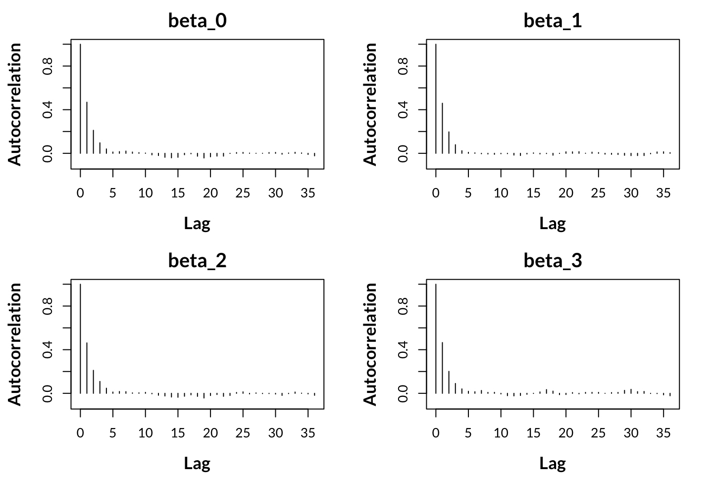
Thinning is a process that is done to help reduce the autocorrelation present in the chains; if there is severe autocorrelation, then the results are not usable for inference. Autocorrelation in the chains is usually diagnosed with an autocorrelation plot. Looking at the autocorrelation for (c), we can see that there is still some concerning autocorrelation (we want almost no spikes for the first half dozen lags); thus, via bumping up the argument thinning to be something higher than 20, say 40, we might resolve the issue of autocorrelation.

old_par <- par()
par(mfrow = c(2,2), mar = c(4.5, 4.5, 2.5, 2),font.lab = 2)
xacf <- list()
for (i in 1:4){
xacf[[i]] <- acf(mcmc.out$chains[[1]][, i], plot = FALSE)
plot(xacf[[i]]$lag,xacf[[i]]$acf, type = "h", xlab = "Lag",ylab = "Autocorrelation", ylim = c(-0.1, 1),cex.lab = 1.3, main = par_names[i], cex.main = 1.5)
}
par(old_par)

Autocorrelation Plot for (c): 1 chain, first four parameters

Mixing of Chains §

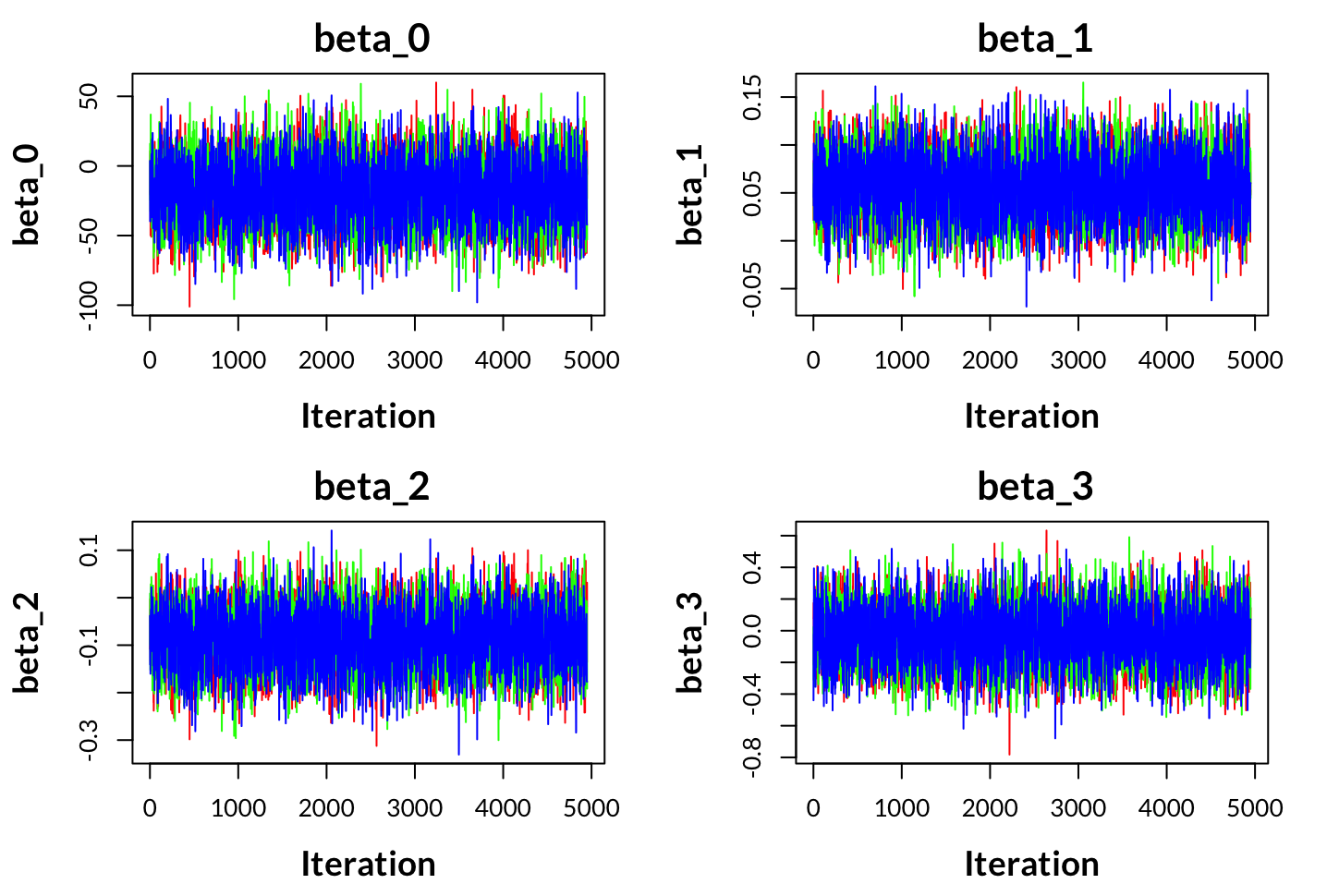
With adding multiple chains, we have just added an extra loop (in this case, iterating over j) to repeat the same sampling procedure for each chain. The traceplots below show good mixing for the first four parameters. If the respective traceplots for each parameter show good mixing of chains, this indicates that the MCMC algorithm converged, and given no problems of autocorrelation, the results are usable for inference.

Traceplot for (c): 3 chains, first four parameters

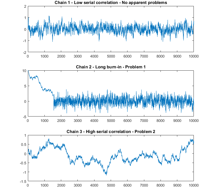
For reference, the image below shows a good mixing of the first chain, indicating convergence, while chain 2 initially shows the chain has not converged until around iteration 1500 and chain 3 never converges. However, a caveat of this plot is that the chains are on different plots. Ideally you want to use a traceplot that shows all chains for a respective parameter on the same plot. Hence, the word mixing is referring to the fuzzy caterpillar-looking image shown in Traceplot for (c)

(Taboga, Marco, 2021)⁵

 

When are MCMC results usable?

If MCMC did not converge, the results are not usable; results are also not usable if there is high autocorrelation shown in the autocorrelation plot.

Adaptive Scaling §

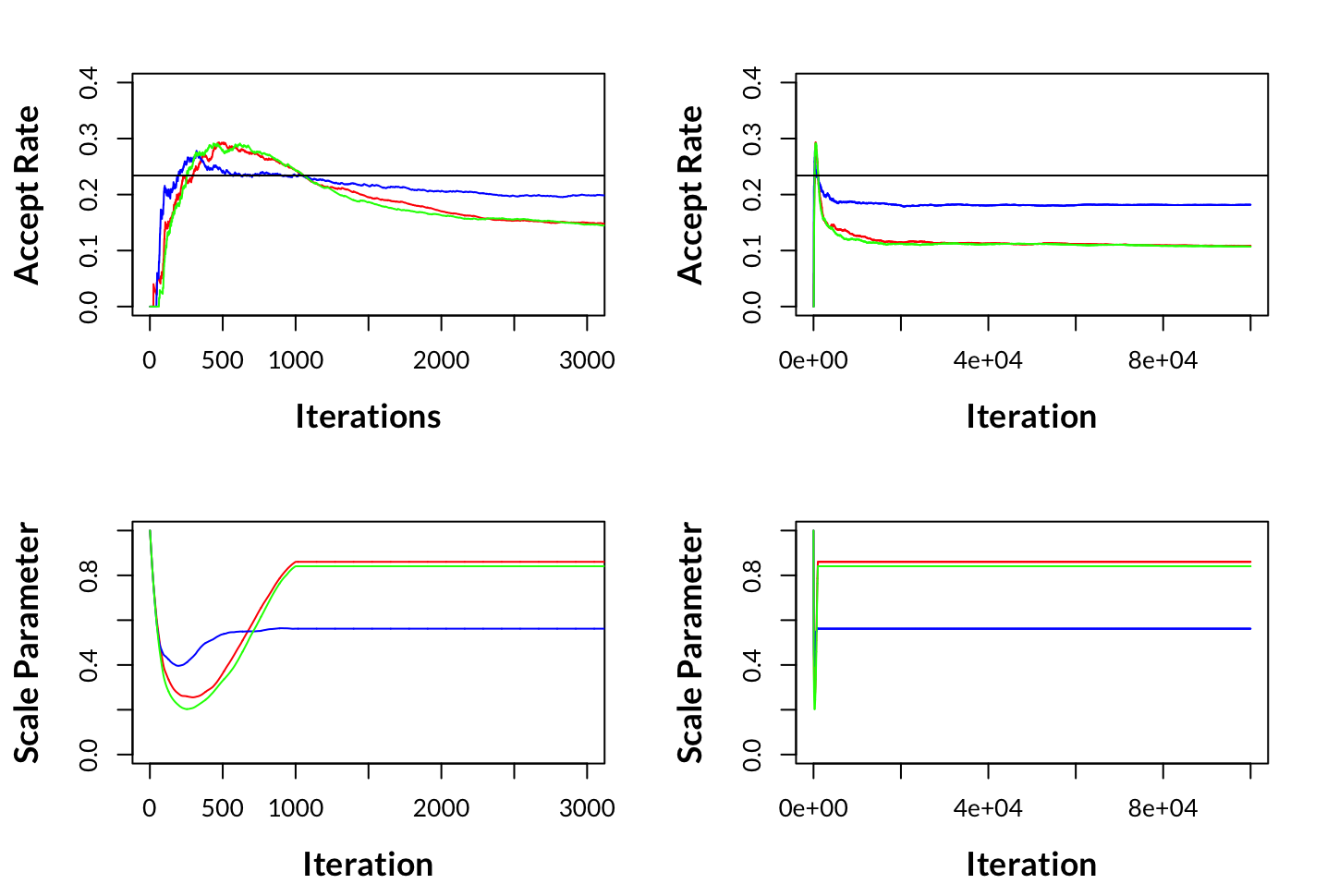
Adaptive Scaling is a hand-off approach to adjusting a scaling term (which I named scale_par i the code), which in terms scales the variance-covariance matrix C. The purpose of this scaling is specific to the accept-reject methodology inherent in Metropolis-Hastings MCMC. As there is no knowing what the Acceptance rate will be before running the algorithm as the process is stochastic and is subject to your data, likelihood, and priors. Notice in Implementation (a) we set scale_par, but in practice, this involved rerunning MCMC multiple times adjusting scale_par each run, trying to get an acceptance rate close to the ideal acceptance rate of 0.234. As shown in MCMC Acceptance Rate Scale Parameter for (c).

Now we are adjusting scale_par dynamically based on the acceptance rate of the proposals during the sampling process. The idea is to increase scale_par if the acceptance rate is too high (indicating that the chain is making too many small, cautious steps) and decrease it if the acceptance rate is too low (indicating that the chain is making too many large, risky steps). scale_par is adapted during the burn-in period. The adaptation is based on the difference between the current acceptance rate and the target acceptance rate (target_acc_rate of 0.234). The learning_rate controls the speed of adaptation. After the burn-in period, the scale_par remains constant for the rest of the sampling. This approach should help achieve a better balance between exploration and exploitation in the parameter space, improving the efficiency of the MCMC chain.

However, there is a caveat: after burn-in, scale_par is no longer being adjusted, and yet the acceptance rate continues to drift below 0.0234 until each of the chains converges. Perhaps you might think to yourself, “Then why don’t you leave scale_par to be adjusted after burn-in as well, then our acceptance rate will still hover close to 0.234”; no doubt some readers will know the answer. We can’t continue to adjust scale_par after burn-in, or we would be breaking the Markov Property subsequently, making our results theoretically invalid; moreover, the chains might never converge if C was continually adjusted by scale_par.

The Markov Property

One of the fundamental properties of MCMC algorithms is the Markov property, which states that the next state of the chain depends only on the current state and not on how it arrived there.

$$P\left(X_{t+n}=x\mid X_t,X_{t-1},\dots ,X_{t-k}\right)=P\left(X_{t+n}=x\mid X_t\right)$$

Hence, adaptive scaling is not perfect; although we can lift the acceptance rate from minuscule digits below 0.001 to above 0.1 (see the top right plot of MCMC Acceptance Rate Scale Parameter for (c)), we still don’t land within a very close distance of the ideal acceptance rate of 0.234. Really, what we have achieved is giving the chains a better starting location post-burn-in in terms of acceptance rates so that when it does converge, it’s hopefully a stone’s throw away from 0.234. From my research, other Adaptive scaling methods have the same problem (see RAM).

MCMC Acceptance Rate Scale Parameter: iterations 0 to 3000 and 0 to 100000

Note

A more popular method for Adaptive scaling is Robust Adaptive Metropolis (RAM). However, to avoid the need for Adaptive Scaling altogether, Gibbs Sampling is another very popular MCMC procedure that uses conditioning to avoid an acceptance rate and, subsequently, the need for Adaptive Scaling.

Resources §

All of the code is available in the directory content/scripts/Metropolis_Hastings_MCMC_from_Scratch at my repo, with bonus content of implementations (d), and (e).

Footnotes §

1. Introna, Michele, et al, 2022 ↩

2. Givens and Hoeting, 2006 ↩

3. Lohman, T, 1992 ↩

4. Roberts and Rosenthal, 2001 ↩

5. Taboga, Marco, 2021 ↩